A Complete Example

Importing laspy

import laspy

Reading .LAS Files

The first step for getting started with laspy is to read a file using the laspy.read() which will give you a LasData object with all the LAS/LAZ content of the source file parsed and loaded.

As the file “simple.las” is included in the repository, the tutorial will refer to this data set. We will also assume that you’re running python from the root laspy directory; if you run from somewhere else you’ll need to change the path to simple.las.

The following short script does just this:

import laspy
las = laspy.read("./tests/data/data/simple.las")

This function reads all the data in the file into memory.

Accessing Data

Now you’re ready to read data from the file. This can be header information, point data, or the contents of various VLR records. In general, point dimensions are accessible as properties of the main file object, and header attributes are accessible via the header property of the main file object. Refer to the background section of the tutorial for a reference of laspy dimension and field names.

# Grab just the X dimension from the file, and scale it.

def scaled_x_dimension(las_file):
    x_dimension = las_file.X
    scale = las_file.header.scales[0]
    offset = las_file.header.offsets[0]
    return (x_dimension * scale) + offset

scaled_x = scaled_x_dimension(las)

Note

Laspy can actually scale the x, y, and z dimensions for you. Upper case dimensions (las_file.X, las_file.Y, las_file.Z) give the raw integer dimensions, while lower case dimensions (las_file.x, las_file.y, las_file.z) give the scaled value. Both methods support assignment as well, although due to rounding error assignment using the scaled dimensions is not recommended.

The LasData object las has a reference to the LasHeader object, which handles the getting and setting of information stored in the laspy header record of simple.las.

Notice also that the scales and offsets values returned are actually arrays of [x scale, y scale, z scale] and [x offset, y offset, z offset] respectively.

LAS files differ in what data is available, and you may want to check out what the contents of your file are. Laspy includes several methods to document the file specification, based on the PointFormat.

# Find out what the point format looks like.
for dimension in las.point_format.dimensions:
    print(dimension.name)

# It looks like we have color data in this file, so we can grab:
blue = las.blue

Many tasks require finding a subset of a larger data set. Luckily, numpy makes this very easy. For example, suppose we’re interested in finding out whether a file has accurate min and max values for the X, Y, and Z dimensions.

import laspy
import numpy as np

las = laspy.read("./tests/data/data/simple.las")
# Some notes on the code below:
# 1. las.header.maxs returns an array: [max x, max y, max z]
# 2. `|` is a numpy method which performs an element-wise "or"
#    comparison on the arrays given to it. In this case, we're interested
#    in points where a XYZ value is less than the minimum, or greater than
#    the maximum.
# 3. np.where is another numpy method which returns an array containing
#    the indexes of the "True" elements of an input array.

# Get arrays which indicate invalid X, Y, or Z values.
X_invalid = (las.header.mins[0] > las.x) | (las.header.maxs[0] < las.x)
Y_invalid = (las.header.mins[1] > las.y) | (las.header.maxs[1] < las.y)
Z_invalid = (las.header.mins[2] > las.z) | (las.header.maxs[2] < las.z)
bad_indices = np.where(X_invalid | Y_invalid | Z_invalid)

print(bad_indices)

Now lets do something a bit more complicated. Say we’re interested in grabbing only the points from a file which are within a certain distance of the first point.

# Grab the scaled x, y, and z dimensions and stick them together
# in an nx3 numpy array

coords = np.vstack((las.x, las.y, las.z)).transpose()

# Pull off the first point
first_point = coords[0,:]

# Calculate the euclidean distance from all points to the first point

distances = np.sqrt(np.sum((coords - first_point) ** 2, axis=1))

# Create an array of indicators for whether or not a point is less than
# 500000 units away from the first point

mask = distances < 500

# Grab an array of all points which meet this threshold

points_kept = las.points[mask]

print("We kept %i points out of %i total" % (len(points_kept), len(las.points)))

As you can see, having the data in numpy arrays is very convenient. Even better, it allows one to dump the data directly into any package with numpy/python bindings. For example, if you’re interested in calculating the nearest neighbors of a set of points, you can use scipy’s KDTtree (or cKDTree for better performance)

import laspy
from scipy.spatial import cKDTree
import numpy as np

las = laspy.read("./tests/data/data/simple.las")
# Grab a numpy dataset of our clustering dimensions:
dataset = np.vstack((las.X, las.Y, las.Z)).transpose()
# Build the KD Tree
tree = cKDTree(dataset)
# This should do the same as the FLANN example above, though it might
# be a little slower.
neighbors_distance, neighbors_indices = tree.query(dataset[100], k=5)
print(neighbors_indices)
print(neighbors_distance)

For another example, lets say we’re interested only in the last return from each pulse in order to do ground detection. We can easily figure out which points are the last return by finding out for which points return_num is equal to num_returns.

# Grab the return_num and num_returns dimensions
ground_points = las.points[las.number_of_returns == las.return_number]

print("%i points out of %i were ground points." % (len(ground_points),
        len(las.points)))

Since the data are simply returned as numpy arrays, we can use all sorts of analysis and plotting tools. For example, if you have matplotlib installed, you could quickly make a histogram of the intensity dimension:

import matplotlib.pyplot as plt
plt.hist(las.intensity)
plt.title("Histogram of the Intensity Dimension")
plt.show()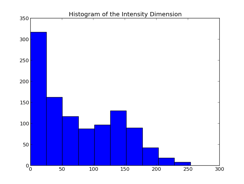

Writing Data

Once you’ve found your data subsets of interest, you probably want to store them somewhere. How about in new .LAS files?

Creating a LasData can be done by using its constructor which expects a LasHeader whether created from scratch or from an input file. Or by using the laspy.create().

# Create a new LasData from the header of the input file
sub_las = laspy.LasData(las.header)
sub_las.points = points_kept.copy()
sub_las.write("close_points.las")

ground_las = laspy.LasData(las.header)
ground_las.points = ground_points.copy()
ground_las.write("ground_points.las")

For another example, let’s return to the bounding box script above. Let’s say we want to keep only points which fit within the given bounding box, and store them to a new file:

import laspy
import numpy as np

las = laspy.read("tests/data/data/simple.las")

# Get arrays which indicate VALID X, Y, or Z values.

X_invalid = (las.header.min[0] <= las.x) & (las.header.max[0] >= las.x)
Y_invalid = (las.header.min[1] <= las.y) & (las.header.max[1] >= las.y)
Z_invalid = (las.header.min[2] <= las.z) & (las.header.max[2] >= las.z)
good_indices = np.where(X_invalid & Y_invalid & Z_invalid)
good_points = las.points[good_indices].copy()

output_file = laspy.LasData(las.header)
output_file.points = good_points
output_file.write("good_points.las")

Variable Length Records

Variable length records, or VLRs, are available in laspy via LasData.vlrs. of a LasData or LasHeader.

This property will return a list of laspy.VLR instances.d. For a summary of what VLRs are, refer to the “Defined Variable Length Records” section of the LAS specification.

To create a VLR, you really only need to know user_id, record_id, and the data you want to store in VLR_body (For a fuller discussion of what a VLR is, see the background section). The rest of the attributes are filled with null bytes or calculated according to your input, but if you’d like to specify the reserved or description fields you can do so with additional arguments.

import laspy

las = laspy.read("./tests/data/data/simple.las")
# Instantiate a new VLR.
new_vlr = laspy.VLR(user_id="The User ID", record_id=1,
              record_data=b"\x00" * 1000)
# Do the same thing, but add a description field.
new_vlr = laspy.VLR("The User ID",1,
                description = "A description goes here.",
                record_data=b"\x00" * 1000,)

# Append our new vlr to the current list. As the above dataset is derived
# from simple.las which has no VLRS, this will be an empty list.
las.vlrs.append(new_vlr)
las.write("close_points.las")